In machine learning and artificial intelligence, adversarial attacks have gained much attention from researchers. These attacks alter the inputs to mislead the model into making wrong predictions. Among these, the Fast Gradient Sign Method (FGSM), is particularly worth mentioning because of its effectiveness and simplicity.
Need more GPU power for this project?
Dedicated NVIDIA GPUs (RTX A4000 to A100) from German data centers – from €92.59/month, billed by the hour, ready in minutes. Rent a GPU server →
Significance of FGSM
The significance of FGSM lies in its ability to expose the vulnerability of modern models to minor variations in input data. These perturbations, which frequently go unnoticed by human observers, inflict errors on prediction accuracy. Understanding and minimizing these vulnerabilities is pivotal to building fault-resistant machine learning systems trusted in practical applications like autonomous driving, healthcare provisioning, and security management.
This compelling article takes a deep dive into the meaning of FGSM and elucidates its mathematical foundations with clarity and precision. It provides demonstrations through an illustrative case study.
First-Order Taylor Expansion in Adversarial Attacks
The utilization of the First-Order Taylor Expansion technique in approximating the loss function is a significant method to understand how slight changes in input can affect the loss in machine learning models. This approach, particularly useful when dealing with adversarial attacks, involves computing an approximation of L(x+δ) using its gradient with Taylor expansion around x:
L(x+δ) ≈ L(x) + ∇L(x) ⋅ δ
The loss at the original input x is denoted as L(x), the gradient of the loss function at x is represented by ∇L(x), and δ is a small perturbation to x. The direction and rate of the steepest increase of the loss function is represented by ∇L(x). By perturbing x in the direction of ∇L(x), we can predict how the loss function will change.
Adversarial attacks use the Taylor Expansion to find perturbations δ that maximize the loss function L(x+δ). This is achieved by choosing δ proportional to the sign of ∇L(x):
δ = ϵ ⋅ sign(∇L(x))
where ϵ is a small scalar controlling the magnitude of the perturbation.
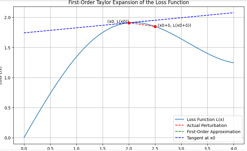
For illustration purpose, let’s draw a diagram to represent the First-Order Taylor Expansion of the loss function. This will include the loss curve, the original point, the gradient vector, the perturbed point, and the first-order approximation.
First-Order Taylor Expansion of the Loss Function
The diagram generated illustrates the key concepts of the First-Order Taylor Expansion of the loss function. Here are the main takeaways:
- Loss Curve (L(x)): A smooth curve representing the loss function over different inputs.
- Original Point (x0, L(x0)): The point on the loss curve which corresponds to the value of the input x0.
- Gradient Vector (∇L(x0)): This represents the slope of the tangent line at the point L(x0).
- Perturbed Point (x0 + δ, L(x0 + δ)): The new point after adding a small perturbation δ to the input x0.
- First-Order Approximation (L(x0) + ∇L(x0) ⋅ δ): The linear approximation of the loss function around x0.
FGSM Adversarial Attack Process
We can see how the gradient of the loss function can be used to approximate the change in loss due to small perturbations in the input. This understanding is crucial for generating adversarial examples in the context of adversarial attacks.
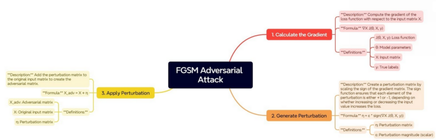
The Fast Gradient Sign Method (FGSM) is based on the principle of using the gradients of the loss function with respect to the input data to determine the direction in which the input should be modified to increase the model’s error. The steps involved in FGSM can be described in the image below:
FGSM Adversarial Attack Process
This process begins by determining the gradient of the loss function with respect to the input data. The gradient defines how the loss function would change if the input data were slightly modified. Understanding this relationship, we can define the direction in which small shifts in inputs will increase the loss.
Once the gradient is computed, the next step is to generate the perturbation. This is achieved through scaling the sign of the gradient. The sign function ensures that each component of the perturbation matrix is either + or - 1. This indicates whether the loss is most sensitive to an increase or a decrease of the corresponding input value.
A scaling factor ensures that these perturbations should be small but large enough to fool the model.
The last step is to generate the adversarial example by applying this perturbation to the original input. By adding the perturbation matrix to the original input matrix, we get the input that looks very similar to the original data but is built to mislead the model into making incorrect predictions.
Uses and Importance of FGSM in Machine Learning
- Testing Model Robustness: FGSM is used to assess machine learning model resilience by testing it against adversarial attacks.
- Improving Model Security: Robust models are key in security applications like self-driving, healthcare, and finance.
- Adversarial Training: It helps in adversarial training, improving model robustness.
- Understanding Model Behavior: FGSM helps understand model behavior during input perturbations.
- Benchmarking Adversarial Defense Techniques: It is used to compare defense techniques against adversarial attacks.
- Educational Purposes: FGSM serves as a basic introduction to adversarial attacks and defenses in machine learning.
Practical Implementation
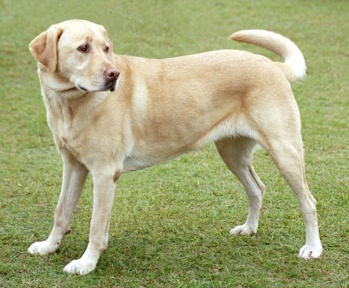
To exemplify the Fast Gradient Sign Method (FGSM) attack practically, we will use TensorFlow to generate adversarial examples. We will use Gradio as an interactive display tool to showcase the results. We’ll use an image of a yellow Labrador retriever, which can be found here.
First, let’s load the necessary libraries and the image:
import tensorflow as tf
import numpy as np
import matplotlib.pyplot as plt
import gradio as gr
import requests
from PIL import Image
from io import BytesIO

# Load the image
image_url = "https://storage.googleapis.com/download.tensorflow.org/example_images/YellowLabradorLooking_new.jpg"
response = requests.get(image_url)
img = Image.open(BytesIO(response.content))
img = img.resize((224, 224))
img = np.array(img) / 255.0

# Display the image
plt.imshow(img)
plt.show()
Output:
FGSM Attack Function
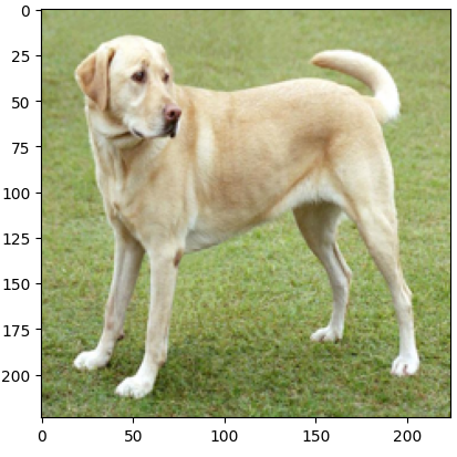
The above Python code helps to load and view an image from a specific URL by using frameworks such as TensorFlow, NumPy, Matplotlib, and PIL. It uses the requests library to fetch the image, resizes it to a 224*224, and normalizes the value of pixels between 0 and 1, before converting the image into a numpy array.
Finally, users can display the image and ensure the program correctly loads and processes the image.
Next, let’s load a pre-trained model and define the FGSM attack function:
# Load a pre-trained model
model = tf.keras.applications.MobileNetV2(weights='imagenet')

# Define the FGSM attack function
def fgsm_attack(image, epsilon):
    image = tf.convert_to_tensor(image, dtype=tf.float32)
    image = tf.expand_dims(image, axis=0)

    with tf.GradientTape() as tape:
        tape.watch(image)
        prediction = model(image)
        loss = tf.keras.losses.categorical_crossentropy(tf.keras.utils.to_categorical([208], 1000), prediction)

    gradient = tape.gradient(loss, image)
    signed_grad = tf.sign(gradient)
    adversarial_image = image + epsilon * signed_grad
    adversarial_image = tf.clip_by_value(adversarial_image, 0, 1)

    return adversarial_image.numpy().squeeze()

# Display the adversarial image
adversarial_img = fgsm_attack(img, epsilon=0.08)
plt.imshow(adversarial_img)
plt.show()
Output:
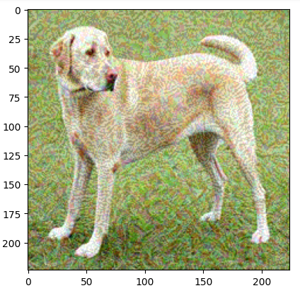
The code above demonstrates how to use the FGSM adversarial attack on an image. It begins by downloading a pre-train mobileNetV2 model with Imagenet weights.
The fgsm_attack method is then defined to perform the adversarial attack. It transforms the input image into a tensor, performs the computational work to determine the model’s prediction, and computes the loss with respect to the target label. By using TensorFlow’s gradient tape, the loss with respect to the image input is computed, and its sign is used to create perturbation. This is added to the original image with a multiplicative factor of epsilon to get an adversarial image. The adversarial image is then clipped to remain in the valid pixel range.
Integrating FGSM with Gradio for Interactive Exploration
Finally, let’s integrate this with Gradio to allow interactive exploration of the adversarial attack:
# Define the Gradio interface
def generate_adversarial_image(epsilon):
    adversarial_img = fgsm_attack(img, epsilon)
    return adversarial_img

interface = gr.Interface(
    fn=generate_adversarial_image,
    inputs=gr.Slider(minimum=0.0, maximum=0.1, value=0.01, label="Epsilon"),
    outputs=gr.Image(type="numpy", label="Adversarial Image"),
    live=True
)

# Launch the Gradio interface
interface.launch()
Output:
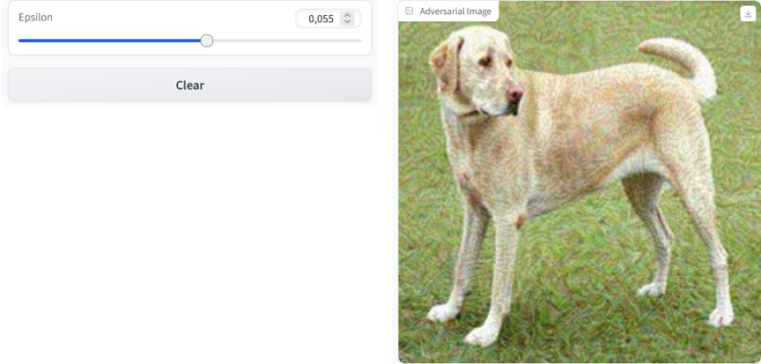
The code above generates a generate_adversarial_image function. It accepts the epsilon value as its parameter and executes the FGSM attack on the image, then outputs the adversarial image.
Our Gradio interface is customized with a slider input that allows for modification of the epsilon value while also showing updates in real-time via live=True parameter setting.
The command interface.launch() starts the web-based Gradio platform where users can manipulate various degrees of values. This enables them to see corresponding adverse images generated by their inputs until they find what suits them best.
Comparison Between FGSM and Other Adversarial Attack Methods
The table below summarizes the comparison between FGSM and other adversarial attack methods:
| Attack Method | Description | Pros | Cons |
|---|---|---|---|
| FGSM | Simple, efficient, uses gradient sign to generate adversarial examples | Quick, easy to implement, good for initial vulnerability assessment | Produces easily detectable perturbations, less effective against robust models |
| PGD | Iterative version of FGSM, refines perturbations over multiple steps | More effective at finding adversarial examples, harder to defend against | Computationally expensive, time-consuming |
| CW | Carlini & Wagner attack, minimizes perturbations to be less detectable | Very effective, produces minimal perturbations | Complex to implement, computationally intensive |
| DeepFool | Finds minimal perturbations to move input across decision boundary | Produces small perturbations, effective for many models | More computationally expensive than FGSM, less intuitive |
| JSMA | Jacobian-based Saliency Map Attack, targets specific pixels for perturbation | Effective at creating targeted attacks, can control which pixels are modified | Complex, can be slow, requires detailed understanding of model |
FGSM is preferred for fast computation and simplicity in carrying out preliminary robustness tests and adversarial learning. In contrast, to create powerful adversarial examples, methods such as PGD or C&W can be used although they are computationally expensive. Methods like DeepFool and JSMA are more suitable for observing minimal perturbations and feature importance but consume more computational power.
Conclusion
This article explores the Fast Gradient Sign Method (FGSM), a crucial technique in adversarial machine learning. This method exposes neural networks’ vulnerabilities to minor input alterations by computing gradients with respect to the loss function. The resulting perturbations can drastically impact model predictions. This makes understanding FGSM’s mathematical foundation crucial to creating resilient machine learning systems that don’t buckle under attack. It’s important to imbue our critical applications with a robust defense mechanism against such attacks.
The practical implementation using TensorFlow and Gradio illustrates FGSM’s real-world application. Users can easily tinker with varying epsilon values to witness how these adjustments shape adversarial image output. Such an example serves as a stark reminder of FGSM’s efficiency while equally underlining AI system vulnerability to malicious attacks. There is a need for robust security measures that guarantee optimal safety and reliability in systems’ operations.
Test your setup on ccloud³
Sign up for ccloud³ and receive €200 starting credit for your project.