
Random Forest Algorithm in Machine Learning: How It Works and Why It Matters
Among the most widely used algorithms in machine learning is Random Forest, a method applied to both classification and regression tasks. It often delivers strong accuracy, which is why it remains one of the most preferred approaches for classification problems. A Random Forest is created by combining many Decision Trees. Generally, the more trees included, the stronger and more refined the overall model becomes. Each tree produces its own prediction, and the final output is determined by majority voting—an approach that improves stability and resilience. In this article, we explore what happens inside a Random Forest and then implement it in Python to gain hands-on familiarity with how it operates.
Why Random Forest?
Random Forest is a supervised learning algorithm most commonly used for classification. In supervised learning, the model learns from labeled examples, which provides guidance during training. One major advantage of Random Forest is its flexibility: it works well for both classification and regression. It functions by blending the outputs of multiple decision trees to produce accurate predictions. Even though using many trees might sound like it could cause overfitting, the method usually avoids that issue. The algorithm chooses the outcome predicted most often across the trees (majority vote), leading to dependable, strong, and versatile performance. In the next sections, we examine how Random Forests are built and how they reduce the weaknesses found in single decision trees.
Disadvantages of Decision Trees
A decision tree is a classification model that creates a defined set of rules describing relationships among data points. Observations (data points) are split based on an attribute so that the resulting groups are as distinct as possible, while members inside each group remain as similar as possible. Put differently, the inter-class distance should be low and the intra-class distance should be high. This is achieved using methods such as Information Gain, Gini Index, and others.
Several limitations can make decision trees harder to apply smoothly, including:
- Overfitting risk in deep trees: Decision trees can overfit when they grow too deep. As splitting continues, more and more attributes are considered. The tree attempts to perfectly match the training set, which causes it to learn too many specifics about the training data and weakens its ability to generalize.
- Greedy, locally optimal splitting: Decision trees are greedy and often settle for locally optimal choices instead of the globally best ones. At each step, a method is used to choose the best split, but the best local split may not lead to the best overall tree. Random Forest helps address these issues.
From Decision Trees to Random Forests
The Problem with Single Decision Trees
Decision Trees are straightforward to use, but they often run into overfitting, high variance, or bias—especially when the tree is too deep or too shallow. A single tree may also produce incorrect predictions if it learns from noisy or biased data.
The Idea of Using Multiple Trees
To solve these problems, researchers suggested merging many trees into one stronger model—an ensemble. This concept was introduced by Tin Kam Ho in 1995 at Bell Laboratories, which laid the foundation for the Random Forest algorithm.
Power of the Forest
A collection of trees (a forest) can compensate for individual errors. If one tree predicts incorrectly, others may predict correctly. When their outputs are combined, the forest delivers a more accurate and more stable prediction. To understand classification with Random Forest, note that each tree casts a “vote” for a class label. The label receiving the most votes becomes the final result. For regression tasks, each tree produces a numeric prediction, and the final output is the average of all predictions.
Randomness Adds Strength
Rather than always selecting the best feature at every split (as a Decision Tree does), Random Forest chooses features randomly. This makes the trees less similar to each other and helps reduce overfitting.
The Role of Bagging (Bootstrap Aggregating)
Random Forest relies on a method called Bagging, short for Bootstrap Aggregation. With bagging, multiple datasets are produced by randomly sampling from the original dataset with replacement. Each sampled dataset trains its own Decision Tree, which reduces variance and boosts accuracy by combining results from all trees.
Feature Bagging – The Random Forest Twist
Random Forest extends bagging by randomizing not only the sampled data but also the features. Each tree receives its own subset of features—this is called feature bagging. This prevents trees from becoming too similar and increases diversity across the forest.
Why It Works So Well
By mixing random data sampling, random feature selection, and multiple trees, the model becomes more resistant to noise, less likely to overfit, and more accurate than a single decision tree.
Difference between Decision Trees and Random Forests
| Feature | Decision Tree | Random Forest |
|---|---|---|
| Core Concept | Builds a single tree structure by creating decision rules based on input features. | Constructs multiple decision trees using random subsets of data and features as part of an ensemble learning approach. |
| Feature Selection | Selects the optimal feature for each split using metrics such as Gini impurity or entropy. | Chooses a random subset of features at each split to increase diversity among trees. |
| Prediction Method | Generates predictions using one decision tree. | Combines predictions from many trees using majority voting (classification) or averaging (regression). |
| Overfitting Risk | More prone to overfitting, especially with deep trees or limited datasets. | Low – randomness and averaging reduce the chance of overfitting. |
| Accuracy | Typically lower accuracy because of higher variance and sensitivity to training data. | Usually achieves higher accuracy through aggregated predictions from multiple trees. |
| Interpretability | Easy to understand and visualize, with transparent decision-making rules. | More difficult to interpret because predictions come from many combined trees. |
| Computational Complexity | Computationally lightweight since only a single tree is trained. | More computationally intensive because multiple trees must be trained and evaluated. |
| Training Speed | Faster to train with fewer calculations required. | Slower training process due to the creation of many trees. |
| Handling Noise and Variance | Sensitive to noisy data and small dataset changes, which may alter the tree structure significantly. | More robust against noise and variance because ensemble diversity stabilizes predictions. |
| Dataset Suitability | Works well with small to medium-sized datasets. | Performs especially well on larger datasets with many features. |
| Typical Use Cases | Suitable for interpretable models and straightforward decision-support systems. | Commonly used for high-accuracy tasks such as fraud detection, risk analysis, and medical diagnostics. |
Applications of Random Forests
The Random Forest classifier is broadly applied in fields such as banking, medicine, and e-commerce because of its strong classification performance, which has driven greater adoption over time. It is used to identify customer behavior patterns, support remote sensing tasks, and evaluate stock market trends. In healthcare, it helps detect pathologies by spotting recurring patterns, and in finance, it plays an important role in separating fraudulent activity from legitimate behavior.
Understanding the Inner Workings of Random Forest: Training, Prediction & Evaluation
Like most Machine Learning algorithms, Random Forest includes two main phases: training and testing. One stage involves creating the forest, and the other stage generates predictions from test data passed into the model. Let’s also consider the mathematical logic that supports the pseudocode.
During training, for each iteration b in 1, 2, … B (where B represents the total number of decision trees), the method starts by applying bagging to produce random subsets of the data. Given a training dataset X and Y, it draws n training examples with replacement to form Xb and Yb. From the full set of available features, N features are randomly chosen, and the best split node n is calculated from that subset. Using the selected split point, the node is divided accordingly. This cycle—choosing features, finding the best split, and splitting nodes—continues until l nodes are produced, and the full process repeats until B trees are created. In testing, predictions for unseen samples x’ are produced by aggregating (averaging) the outputs from all individual regression trees.
For classification, the process gathers votes from every tree, and the class receiving the most votes is treated as the final prediction.
The best number of trees in a Random Forest (B) can be selected based on dataset size, cross-validation, or out-of-bag error. Let’s define these ideas.
Cross-validation is commonly used to reduce overfitting in machine learning. It repeatedly trains on training data and evaluates on different test splits across multiple iterations, represented by k, which is why it is called k-fold cross-validation. This process can guide the choice of how many trees to use based on the k value. Out-of-bag error is the average prediction error for each training sample xi, calculated using only those trees that did not include xi in their bootstrap sample. It resembles a leave-one-out cross-validation approach.
Computing the feature importance (Feature Engineering)
Next, let’s look at how Random Forest can be implemented using the scikit-learn library in Python. A useful first step is evaluating feature importance, which provides a clearer picture of which features influence predictions most. Scikit-learn includes a feature-importance indicator that represents the relative importance of each feature. This value is computed using the Gini Index or Mean decrease in impurity (MDI), which reflects how much impurity is reduced by splits involving that feature across all trees in the forest.
This score shows how much each feature contributes during training and normalizes the values so the total equals 1. As a result, it becomes easier to shortlist key features and remove those that do not meaningfully influence the model (no impact or minimal impact). Limiting the number of features is helpful because it reduces overfitting, which often appears when there are many attributes.
Random Forest for Regression: Predicting Continuous Values
Although Random Forest is often associated with classification, it also performs extremely well in regression settings, where the objective is to estimate a continuous numerical outcome (for example, house prices, temperature values, or sales figures).
How It Works
Rather than selecting a class through voting as in classification, every decision tree in the forest outputs a numerical estimate. The model then produces the final result by averaging the predictions from all trees. This averaging effect lowers variance and typically yields predictions that are both more accurate and more consistent.
Step-by-Step Logic
- Multiple decision trees are trained using random subsets of the dataset (including both rows and columns).
- Each tree outputs a numeric estimate for the given input data point.
- The model combines all tree outputs by averaging them to generate the final result.
If a Random Forest contains B trees and each tree returns a prediction hb(x), then the final prediction ŷ for an input x is:
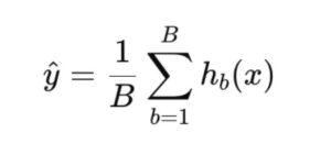
Where:
- hb(x) = prediction from the b-th tree
- B = total number of trees in the forest
- ŷ = final predicted value (average of all trees)
RF can model nonlinear relationships effectively and also lowers overfitting through averaging. In addition, Random Forest regression models tend to be resilient against outliers and can cope well with missing data.
Random Forest Hyperparameters in Scikit-learn
Scikit-learn’s RandomForestClassifier includes multiple adjustable hyperparameters that let you influence the model’s complexity, speed, and accuracy. Below are the most important ones:
1. n_estimators – Number of Trees in the Forest
This defines how many decision trees are built and combined inside the Random Forest. In most cases, increasing the number of trees improves accuracy and stability because more predictions are averaged, reducing variance. However, more trees also increase runtime and memory usage. In scikit-learn, the default was 10 in version 0.20, but starting with version 0.22 it was raised to 100, offering a practical tradeoff between model quality and training efficiency.
2. criterion – Split Quality Function
This setting determines how split quality is measured at each node. The two most common choices are ‘gini’ and ‘entropy’. The ‘gini’ index calculates impurity using the probability that a randomly selected element would be misclassified if it were randomly labeled based on the node’s class distribution. In contrast, ‘entropy’ relies on information gain and reflects how much uncertainty decreases after the split. While ‘gini’ is the default and usually faster, ‘entropy’ may sometimes yield slightly better results depending on the dataset.
3. max_depth – Maximum Tree Depth
The max_depth parameter limits how deep each tree in the forest is allowed to grow. If set to None, splitting continues until all leaves are pure, meaning no further classification improvement is possible. Deep trees can capture complex patterns, but they also increase overfitting risk. Defining a maximum depth helps control overfitting and can also reduce computation time, improving generalization and efficiency.
4. max_features – Features Considered at Each Split
This determines how many features the model evaluates when searching for the best split at each node. For classification, the default is typically ‘auto’ or ‘sqrt’, which uses the square root of the total feature count. Another option is ‘log2’, based on the base-2 logarithm of the feature count. You can also set an integer for an exact feature number or a float (such as 0.5) to represent a fraction of all features. Tuning this value helps balance predictive performance and computational cost. Randomizing features at each split increases tree diversity, which reduces correlation and helps limit overfitting.
5. min_samples_leaf – Minimum Samples in a Leaf Node
This specifies the smallest number of samples required in a leaf node (the terminal node of a tree). Larger values make trees more cautious by discouraging splits that create extremely small leaves, reducing overfitting risk and often improving generalization—especially in noisy or imbalanced datasets. The default value is 1, allowing maximum splitting flexibility but also increasing overfitting potential.
6. n_jobs – Number of Parallel Jobs
This controls how many CPU cores can be used to train the Random Forest in parallel. With None or 1, training runs on a single core. Setting n_jobs=-1 allows the model to use all available cores, which can greatly accelerate training and prediction—particularly for large datasets or forests with many trees.
7. oob_score – Out-of-Bag Evaluation
This Boolean option decides whether out-of-bag (OOB) samples should be used to estimate model performance. OOB samples are those data points that were not included in a tree’s bootstrap sample. When oob_score is True, the model uses these excluded samples like an internal validation set to estimate generalization error. This can reduce the need for separate cross-validation and is especially helpful for large datasets. By default, this setting is False.
Coding the algorithm
Step 1: Exploring the data
First, import the MNIST data from the datasets library available in sklearn.
from sklearn import datasets
mnist = datasets.load_digits()
X = mnist.data
Y = mnist.target
Next, inspect the dataset by printing both the input values (data) and the output labels (target).
[[ 0.  0.  5. 13.  9.  1.  0.  0.  0.  0. 13. 15. 10. 15.  5.  0.  0.  3.
  15.  2.  0. 11.  8.  0.  0.  4. 12.  0.  0.  8.  8.  0.  0.  5.  8.  0.
   0.  9.  8.  0.  0.  4. 11.  0.  1. 12.  7.  0.  0.  2. 14.  5. 10. 12.
   0.  0.  0.  0.  6. 13. 10.  0.  0.  0.]]
[0]
print(mnist.data.shape)
print(mnist.target.shape)

Output:

(1797, 64)
(1797,)
Step 2: Preprocessing the data
This step involves building a DataFrame using Pandas. The target values are stored in y and the input data in X. pd.Series is used to extract a 1D integer array, limited to category values. pd.DataFrame converts the input data into a table format. head() returns the first five rows of the DataFrame. Print them as shown below.
import pandas as pd

y = pd.Series(mnist.target).astype('int').astype('category')
X = pd.DataFrame(mnist.data)

print(X.head())
print(y.head())
Output:

   0    1    2     3     4     5    6    7    8    9  ...    54   55   56  \
0  0.0  0.0  5.0  13.0   9.0   1.0  0.0  0.0  0.0  0.0 ...   0.0  0.0  0.0
1  0.0  0.0  0.0  12.0  13.0   5.0  0.0  0.0  0.0  0.0 ...   0.0  0.0  0.0
2  0.0  0.0  0.0   4.0  15.0  12.0  0.0  0.0  0.0  0.0 ...   5.0  0.0  0.0
3  0.0  0.0  7.0  15.0  13.0   1.0  0.0  0.0  0.0  8.0 ...   9.0  0.0  0.0
4  0.0  0.0  0.0   1.0  11.0   0.0  0.0  0.0  0.0  0.0 ...   0.0  0.0  0.0

    57   58    59    60    61   62   63
0  0.0  6.0  13.0  10.0   0.0  0.0  0.0
1  0.0  0.0  11.0  16.0  10.0  0.0  0.0
2  0.0  0.0   3.0  11.0  16.0  9.0  0.0
3  0.0  7.0  13.0  13.0   9.0  0.0  0.0
4  0.0  0.0   2.0  16.0   4.0  0.0  0.0

[5 rows x 64 columns]
0    0
1    1
2    2
3    3
4    4
dtype: category
Categories (10, int64): [0, 1, 2, 3, ..., 6, 7, 8, 9]
Split the input (X) and output (y) into training and testing sets using train_test_split from sklearn’s model_selection package. test_size indicates that 70% of the dataset is used for training and 30% for testing.
from sklearn.model_selection import train_test_split

X_train, X_test, y_train, y_test = train_test_split(X, y, test_size=0.3)
X_train is the input in the training data.
X_test is the input in the testing data.
y_train is the output in the training data.y_test is the output in the testing data.
Step 3: Creating the Classifier
Train the model using the training dataset with RandomForestClassifier from sklearn’s ensemble package. The n_estimators parameter indicates that 100 trees are included in the Random Forest. The fit() method trains the model using X_train and y_train.
from sklearn.ensemble import RandomForestClassifier

clf=RandomForestClassifier(n_estimators=100)
clf.fit(X_train,y_train)
Generate predictions by applying predict() to the X_test data. The predicted values are stored in y_pred.
y_pred=clf.predict(X_test)
Evaluate accuracy using accuracy_score from sklearn’s metrics package. Accuracy is computed by comparing actual values (y_test) to predicted values (y_pred).
from sklearn.metrics import accuracy_score

print("Accuracy: ", accuracy_score(y_test, y_pred))
Output:
Accuracy:  0.9796296296296
This corresponds to 97.96% estimated accuracy for the trained Random Forest classifier—an excellent result.
Step 4: Estimating the feature importance
Earlier sections highlighted feature importance as a key characteristic of the Random Forest Classifier. Now we compute it.
feature_importances_ is available in sklearn as part of RandomForestClassifier. Extract the values and sort them in descending order so the most influential features appear first.
feature_imp=pd.Series(clf.feature_importances_).sort_values(ascending=False)
print(feature_imp[:10])
Output:
21    0.049284
43    0.044338
26    0.042334
36    0.038272
33    0.034299
dtype: float64
The left column represents the attribute label (for example, the 26th attribute, the 43rd attribute, and so on), while the right column shows the feature-importance value.
Step 5: Visualizing the feature importance
Import matplotlib, pyplot, and seaborn to visualize the feature-importance results. Provide the input and output values where x corresponds to the feature importance values and y corresponds to the 10 most important features out of the 64 attributes.
import matplotlib.pyplot as plt
import seaborn as sns

%matplotlib inline
sns.barplot(x=feature_imp, y=feature_imp[:10].index)
plt.xlabel('Feature Importance Score')
plt.ylabel('Features')
plt.title("Visualizing Important Features")
plt.legend()
plt.show()
Advantages of Random Forest
- Random Forest is a highly versatile and reliable algorithm that performs well across a broad range of machine learning problems.
- It can manage missing values effectively, often reducing the need for explicit data imputation.
- Beyond supervised learning, Random Forest can also be adapted for unsupervised tasks such as clustering by using proximity-based similarity measures.
- The algorithm is relatively straightforward to understand and implement, particularly with machine learning libraries like scikit-learn.
- Even with minimal parameter tuning, Random Forest frequently delivers strong baseline performance.
- By aggregating predictions from multiple independent trees, it significantly reduces the risk of overfitting.
- Random Forest also supports feature importance analysis, making it useful for identifying the most influential variables in a dataset.
- It performs especially well on high-dimensional datasets containing a large number of input features.
Disadvantages of Random Forest
- Training and inference with Random Forest can become computationally expensive, particularly when working with large datasets or many trees.
- The model is less interpretable than a single decision tree because decision logic is distributed across numerous trees within the ensemble.
- Increasing the number of trees often improves accuracy, but it can also significantly extend training time.
- Prediction latency may also increase, which can be a limitation in applications that require fast or real-time responses.
Summary and Conclusion
Random Forest is a strong, beginner-friendly machine learning algorithm that offers a solid balance between simplicity and performance. By blending the strengths of many decision trees, it limits overfitting and produces strong outcomes for both classification and regression tasks. Whether you are working with structured datasets or tackling real-world business challenges, Random Forest remains a reliable choice within the ML toolkit.