
Ridge Regression: Regularization to Reduce Overfitting in Machine Learning
The purpose of machine learning is to develop models that can make reliable predictions beyond the examples used during training. One major challenge is overfitting: a model may achieve impressive results on the training set, yet perform poorly when applied to unseen data. Ridge regression helps reduce this risk by using regularization, which limits overly large coefficients through an added penalty.
This guide provides a complete introduction to Ridge regression. It begins with the basic idea behind the method, then explains the key mathematical principles. You will also see how Ridge compares with related techniques such as Lasso and ElasticNet, followed by a practical Python implementation. Finally, the guide covers useful recommendations and typical situations in which Ridge regression can be especially valuable in practice.
Prerequisites
- Comfort with matrices, eigenvalues, and fundamental optimization ideas, including how to interpret a cost function.
- Knowledge of how overfitting harms model performance and why regularization (penalty terms such as L2) is used to manage it.
- Ability to work with Python libraries such as NumPy, pandas, and scikit-learn, including data preprocessing and model evaluation workflows.
- Understanding of train/test splitting, cross-validation, hyperparameter tuning, and common metrics like R² and RMSE.
- Familiarity with fitting a line or hyperplane and the ordinary least squares method.
What Is Ridge Regression?
Ridge regression extends linear regression by applying ridge regularization. In standard linear regression, the main objective is to find a hyperplane (or a line in two dimensions) that minimizes the total sum of squared errors between the observed values and the predicted values.
Sum of Squared Errors,
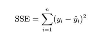
yi denotes the true value of the dependent variable, while ŷi is the corresponding prediction. When the number of predictors is large or features are highly collinear, regression models are more likely to overfit. In overfitting situations, coefficients can become extremely large, causing the model to learn noise and random fluctuations rather than the real relationships in the data.
How Ridge Regression Works?
Ridge Regression limits coefficient magnitudes by adding a penalty term to the sum of squared errors:
Cost Function for Ridge,
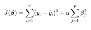
Here:
- βj stands for the parameters or coefficients.
- The regularization parameter α controls how strong the penalty is in the Ridge regression model.
- p is the overall number of parameters in the model.
Classic linear regression computes coefficients by solving the normal equation,
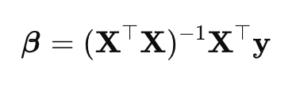
- β is the coefficient vector.
- Xᵀ is the transpose of matrix X.
- (XᵀX)⁻¹ is the inverse of the product XᵀX.
- y is the target vector.
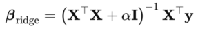
Ridge regression adapts this method by adding a penalty term—specifically I—to XᵀX,
Key Insights
- Shrinkage: When αI is added to XᵀX, the eigenvalues of XᵀX + αI become larger than or equal to those of XᵀX. That makes the matrix more stable to invert and helps prevent oversized coefficient estimates.
- Bias-Variance Trade-off: Shrinking coefficients slightly increases bias but meaningfully lowers variance. This trade can improve performance on new, unseen data.
- Hyperparameter α: α sets the strength of regularization. If it is too large, coefficients may shrink so much that the model underfits. If it is too small, regularization barely helps and the model may overfit, behaving similarly to ordinary linear regression.
Practical Usage Considerations
Strong results with Ridge Regression in practical settings depend on solid data preparation, thoughtful hyperparameter tuning, and careful interpretation of model behavior.
Data Scaling and Normalization
A frequent mistake is ignoring scaling or normalization of feature data. Ridge regression penalizes coefficient sizes to reduce overfitting, but if features sit on different scales, the penalty can be applied unevenly. Large-scale features may have their coefficients shrunk more aggressively than small-scale features, which can produce biased and unstable results.
Standardizing or normalizing the dataset ensures each feature contributes comparably to the penalty term. When features share a similar scale, Ridge regression can penalize coefficients more consistently, improving reliability and overall performance. As a result, a best practice is to standardize or normalize data before applying Ridge regression.
Hyperparameter Tuning
Cross-validation is the standard technique for choosing the best α value, which controls the regularization strength. In most cases, you evaluate a range of alpha values—often spaced logarithmically—fit the model, measure validation performance, and pick the value that produces the best outcome.
Model Interpretability vs. Performance
Ridge regression can reduce interpretability because it does not necessarily remove any features. Coefficients are shrunk but remain present. If interpretability is crucial and many features are irrelevant, it is important to compare Ridge regression to Lasso or ElasticNet.
Avoiding Misinterpretation
A common misconception is treating Ridge regression as a direct feature selection method. Ridge can highlight more influential features because some coefficients shrink less than others, but it does not drive coefficients exactly to zero. If your goal is a model that concentrates on a smaller feature subset, Lasso or ElasticNet may be more appropriate.
Ridge Regression Example and Implementation in Python
The example below shows how to implement Ridge regression with scikit-learn. Imagine a housing-price dataset with features such as house size, bedroom count, age, and location metrics. The aim is to predict price, and we suspect certain predictors might be correlated (for example, house size and number of bedrooms).
Import the required libraries
import numpy as np
import pandas as pd
from sklearn.model_selection import train_test_split, GridSearchCV
from sklearn.preprocessing import StandardScaler
from sklearn.linear_model import Ridge
from sklearn.metrics import r2_score, mean_squared_error
Load the dataset
In a neat tabular layout, features are stored in columns, while the target (price) is kept in its own column. The synthetic dataset imitates patterns commonly seen in real-world data (such as the link between house size and bedroom count).
# --- synthetic--but you could load a real CSV here ---
np.random.seed(42)
n_samples = 200
df = pd.DataFrame({
    "size": np.random.randint(500, 2500, n_samples),
    "bedrooms": np.random.randint(1, 6, n_samples),
    "age": np.random.randint(1, 50, n_samples),
    "location_score": np.random.randint(1, 10, n_samples)
})
# price formula with some noise
df["price"] = (
      df["size"]   * 200
    + df["bedrooms"] * 10000
    - df["age"]      *  500
    + df["location_score"] * 3000
    + np.random.normal(0, 15000, n_samples)      # ← noise
)
Split features and target
Separating predictors (X) from the target (y) clarifies what the model should learn.
X = df.drop("price", axis=1).values
y = df["price"].values
Train-test split
Holding out 20 % of the data for final evaluation can give a realistic picture of how well the model generalizes.
X_train, X_test, y_train, y_test = train_test_split(
X, y, test_size=0.2, random_state=42
)
Standardize the features
The L2 penalty in Ridge uses the squared magnitude of coefficients. Scaling ensures that features with larger numeric ranges do not dominate the penalty.
scaler = StandardScaler()
X_train_scaled = scaler.fit_transform(X_train)
X_test_scaled  = scaler.transform(X_test)
Define a hyperparameter grid for α (regularization strength)
The function np.logspace(-2, 3, 20) creates 20 α values (regularization strengths) spaced logarithmically from 10-2 (0.01) to 103 (1000). This log grid makes it possible to evaluate both weak and strong regularization settings.
param_grid = {"alpha": np.logspace(-2, 3, 20)}  # 0.01 → 1000
ridge = Ridge()
Perform a cross-validation grid search
Cross-validation helps balance bias and variance and reduces the chance of selecting a model due to a fortunate single train-test split.
grid = GridSearchCV(
    ridge,
    param_grid,
    cv=5,                       # 5-fold CV
    scoring="neg_mean_squared_error",
    n_jobs=-1
)
grid.fit(X_train_scaled, y_train)
print("Best α:", grid.best_params_["alpha"])
Output: Best α: 0.01
Because the dataset quality was already strong, only a light amount of regularization was needed. This kept predictions stable without making the model overly simplistic or shrinking coefficients too aggressively.
Selected Ridge Estimator
best_ridge = grid.best_estimator_
best_ridge.fit(X_train_scaled, y_train)
Evaluate the model on unseen data
In the snippet below, R² shows how much of the variation is explained when the model is applied to unseen examples. RMSE reflects the typical gap between predicted and actual house prices, expressed in the same currency units.
y_pred = best_ridge.predict(X_test_scaled)

r2   = r2_score(y_test, y_pred)
mse  = mean_squared_error(y_test, y_pred)  # returns MSE
rmse = np.sqrt(mse)                        # take square root
print(f"Test R²  : {r2:0.3f}")
print(f"Test RMSE: {rmse:,.0f}")
Output: Test R² : 0.988 Test RMSE: 14,229
A test R² of 0.988 indicates the model explains 98.8 % of the price variation for unseen houses. That means the included predictors capture nearly all meaningful price fluctuations.
An RMSE of $14,000 implies that, on average, predictions differ from true values by roughly $14,000.
Inspect the coefficients
Reviewing coefficients that are reduced but still non-zero shows which variables drive house prices while confirming that no feature was removed.
coef_df = pd.DataFrame({
    "Feature": df.drop("price", axis=1).columns,
    "Coefficient": best_ridge.coef_
}).sort_values("Coefficient", key=abs, ascending=False)

print(coef_df)
Output:
| Feature | Coefficient |
|---|---|
| size | 107 713.283911 |
| bedrooms | 14 358.773012 |
| age | -8 595.556581 |
| location_score | 5 874.461993 |
The coefficients suggest that size is the dominant driver of home value, with larger homes gaining about $108,000 per standardized unit increase. Each extra bedroom adds roughly $14,000. As a home ages, value drops by around $8,600 per year. A one-point rise in location score increases the predicted price by about $5,874.
Advantages and Disadvantages of Ridge Regression
The table below summarizes Ridge regression’s primary strengths and limitations.
| Advantages | Disadvantages | Quick Take-away |
|---|---|---|
| Reduces overfitting — the L2 penalty compresses large coefficients, lowering variance and improving generalization. | No built-in feature selection — coefficients never become zero, so the model remains dense. | Pick Ridge when you want to keep every predictor while limiting how strongly each one influences the result. |
| Manages multicollinearity — stabilizes estimates when predictors are strongly correlated. | Hyperparameter tuning needed — the best α typically comes from cross-validation, which can increase compute cost. | Plan time for a CV grid or search across α values. |
| Efficient to compute — provides a closed-form solution and fast, well-established implementations in scikit-learn. | Less interpretable — every feature stays (though reduced), making coefficients harder to read than sparse Lasso models. | Combine Ridge with feature-importance visuals or SHAP to improve clarity. |
| Preserves continuous coefficients — useful when multiple features jointly drive the outcome and none should be removed outright. | Adds bias if α is too high — excessive shrinkage can lead to underfitting and lost signal. | Track validation error as α grows and stop before performance starts to drop. |
Use the guidance above as a fast reference for deciding whether Ridge regression is the right regularization choice for your project.
Ridge Regression vs. Lasso vs. ElasticNet
In machine learning, discussions about regularization typically focus on three main techniques: Ridge regression, Lasso regression, and ElasticNet. Although all three methods aim to reduce overfitting by penalizing large coefficients, they differ in how the penalty is applied and how coefficients are treated.
| Aspect | Ridge Regression | Lasso Regression | Elastic Net |
|---|---|---|---|
| Penalty Type | L2 (sum of squared coefficients) | L1 (sum of absolute coefficients) | Combination of L1 and L2 |
| Effect on Coefficients | Reduces all coefficients; none are forced exactly to 0 | Drives some coefficients exactly to 0 (feature selection) | Pushes some coefficients to 0 while shrinking others |
| Feature Selection | No | Yes | Yes |
| Best For | Large number of predictors, multicollinearity | High-dimensional datasets with only a few relevant variables | Correlated predictors requiring both shrinkage and selection |
| Handling Correlated Features | Spreads weights across correlated variables | Often keeps one variable and discards the others | Can retain groups of correlated variables |
| Interpretability | Lower (all features remain) | Higher (sparse model with fewer predictors) | Moderate |
| Hyperparameters | λ (regularization strength) | λ (regularization strength) | λ (overall strength), α (L1/L2 mixing ratio) |
| Common Use Cases | Price prediction with many correlated inputs | Gene selection, text classification | Genomics, finance, datasets with correlated predictors |
| Limitation | Does not perform feature selection | Can be unstable when predictors are highly correlated | Requires tuning of two hyperparameters |
The choice between Ridge regression, Lasso, and ElasticNet depends on the structure of your dataset and the goals of your task. Ridge regression is especially suitable when predictors are correlated and there is no need to eliminate features. Lasso is preferable when removing irrelevant variables is important. ElasticNet combines both approaches and serves as a balanced alternative.
Applications of Ridge Regression
Ridge Regression supports stable and accurate predictions across many industries, particularly when working with complex or high-dimensional datasets. Below are several practical applications:
- Finance and Economics: Tasks such as portfolio optimization and risk modeling require stable coefficient estimates. Ridge regression helps control extreme fluctuations and improves robustness.
- Healthcare: Diagnostic prediction models can suffer from overfitting and unstable coefficients. Ridge regression enhances model stability and reduces misinterpretation risks.
- Marketing and Demand Forecasting: Forecasting sales or click-through rates often involves numerous highly correlated variables. Ridge regression effectively handles multicollinearity in such cases.
- Natural Language Processing: In text classification and sentiment analysis, thousands of features (words and n-grams) may be present. Ridge regression helps prevent overfitting to unimportant terms and manages correlated predictors efficiently.
FAQ Section
Q1. What is Ridge regression?
Ridge regression is a linear regularization technique that incorporates an L2 penalty, squaring the coefficients to address multicollinearity and reduce overfitting.
How does Ridge regression prevent overfitting?
By penalizing large coefficient values, Ridge regression slightly increases bias while significantly lowering variance, which improves generalization to unseen data.
What is the difference between Ridge and Lasso Regression?
Ridge regression (L2) shrinks coefficients to limit overfitting, whereas Lasso regression (L1) forces certain coefficients to become exactly zero, thereby performing feature selection.
When should I use Ridge Regression over other models?
Ridge regression is ideal for datasets containing many correlated variables where predictive information is distributed across several features and stable estimates are more important than sparsity.
Can Ridge Regression perform feature selection?
No. Ridge regression reduces coefficient magnitudes but does not eliminate features from the model.
How do I implement Ridge Regression in Python?
You can apply Ridge regression using scikit-learn. Begin by importing the Ridge class: from sklearn.linear_model import Ridge.
Create a model, for example: model = Ridge(alpha=1.0). This initializes Ridge regression with an alpha value of 1.0 as the regularization strength.
Train the model using model.fit(X_train, y_train) and generate predictions with model.predict(X_test).
Scikit-learn’s Ridge implementation automatically incorporates the L2 penalty.
For classification problems, you can use LogisticRegression with penalty=’l2′.
Conclusion
Ridge Regression offers a dependable solution for reducing overfitting, especially in datasets characterized by multicollinearity or a large number of predictors. The L2 penalty stabilizes coefficient estimates while retaining all variables, achieving a balance between bias and variance.
With appropriate data preprocessing, careful hyperparameter optimization, and thoughtful interpretation, Ridge regression enhances performance in areas such as finance, healthcare, marketing, and natural language processing.
Knowing when to apply Ridge regression—and how it compares to Lasso and ElasticNet—helps maintain the accuracy, stability, and robustness of machine learning models.